| 1 | Define the purpose and the scope of the benchmark. |
| 2 | Include all relevant methods. |
| 3 | Select (or design) appropriate datasets. |
| 4 | Choose appropriate parameter values and software versions. |
| 5 | Evaluate methods according to key quantitative performance metrics. |
| 6 | Evaluate secondary metrics including computational requirements, user-friendliness, installation procedures, and documentation quality. |
| 7 | Interpret results and provide recommendations from both user and method developer perspectives. |
| 8 | Publish results in an accessible format. |
| 9 | Design the benchmark to include future extensions. |
| 10 | Follow reproducible research best practices, by making code and data publicly available. |
6 Simulation Testing
6.1 Introduction
Testing a proposed model against simulated data generated from a known underlying process is an important but sometimes overlooked step in ecological research (Austin et al. 2006; Lotterhos, Fitzpatrick, and Blackmon 2022). In fisheries science, simulation testing is commonly used to evaluate stock assessment and population dynamic models and assess their robustness to various types of error (Deroba et al. 2015; Piner et al. 2011).
Before applying the size-at-maturity estimation procedures identified through the systematic review to real data, I will create multiple simulated data sets with differing characteristics in order to determine the domains of applicability and inference of each model. The domain of applicability refers to the types of data sets to which a model can reliably be applied, while the domain of inference is defined as the processes or conclusions that can be inferred from the model output (Lotterhos, Fitzpatrick, and Blackmon 2022). The methodology for this chapter will be heavily influenced by the principles for ecological simulation testing outlined by Lotterhos et al. (2022) and the guidelines for computational method benchmarking developed by Weber et al. (2019) (See Box 1).
6.2 Basic simulation steps
- Create a normal distribution of the body size variable
- Calculate probability of maturity for each individual based on body size
- Calculate predicted claw or abdomen size based on body size
- Add error
The fake_crustaceans function in morphmat allows users to rapidly generate many data sets with options for changing parameters in each of the four steps.
In more detail:
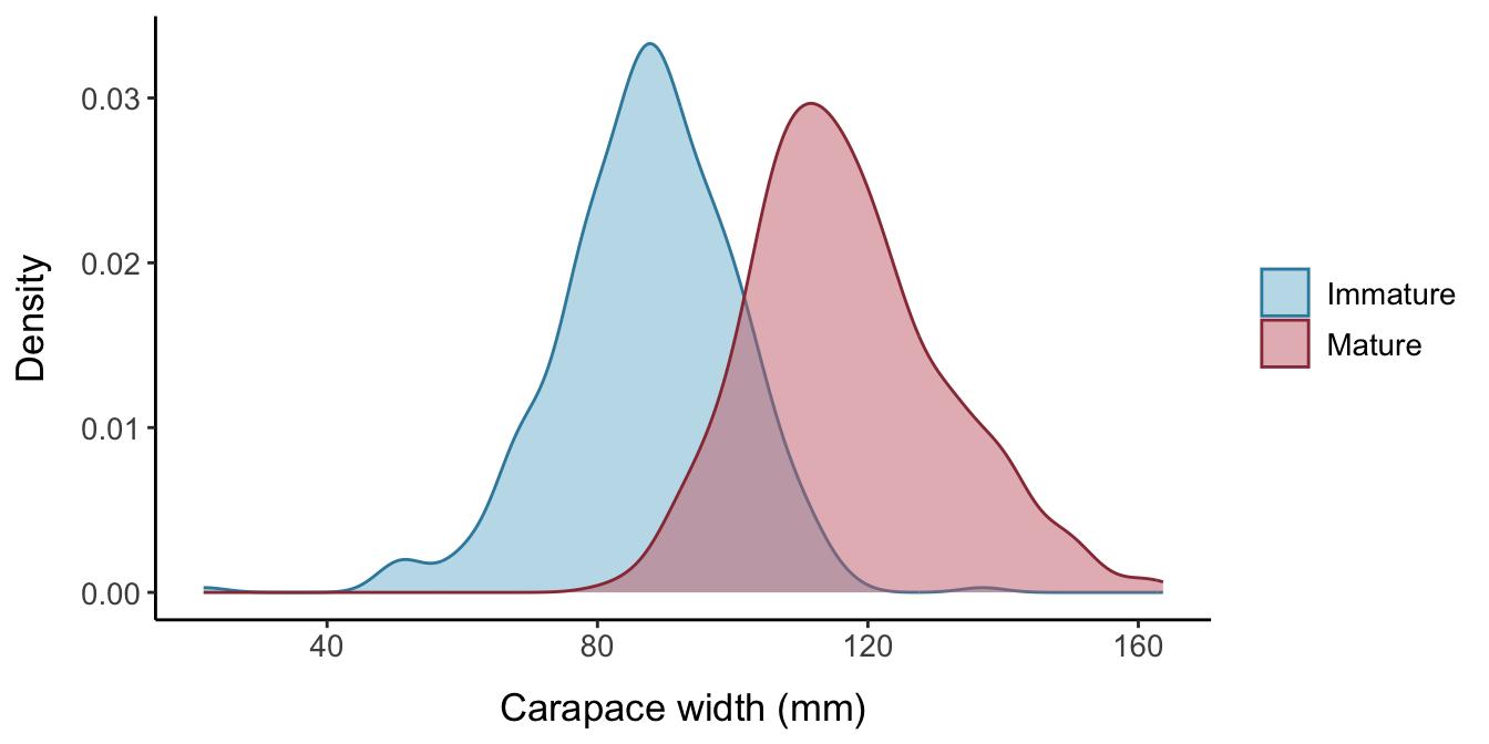
- Create a normal distribution of the body size variable with the specified mean and SD. The
fake_crustaceansdefault is to generate a random sample of 1000 crustaceans with a mean carapace width/body size of 105 mm and standard deviation of 20 mm.

- Use a logistic distribution with known location and scale parameters (i.e., known L50 and steepness of the logistic curve) to find the probability of maturity for each individual based on their body size. The
fake_crustaceansdefault is for the true size at maturity for the population to be 100 mm, with a slope parameter for the logistic equation of 5.
The parameterization of the logistic equation we will use is: \[f(x)=\frac{1}{1+e^{-(x-a)/b}} \] where \(a\) is a location parameter and \(b\) is the shape parameter.
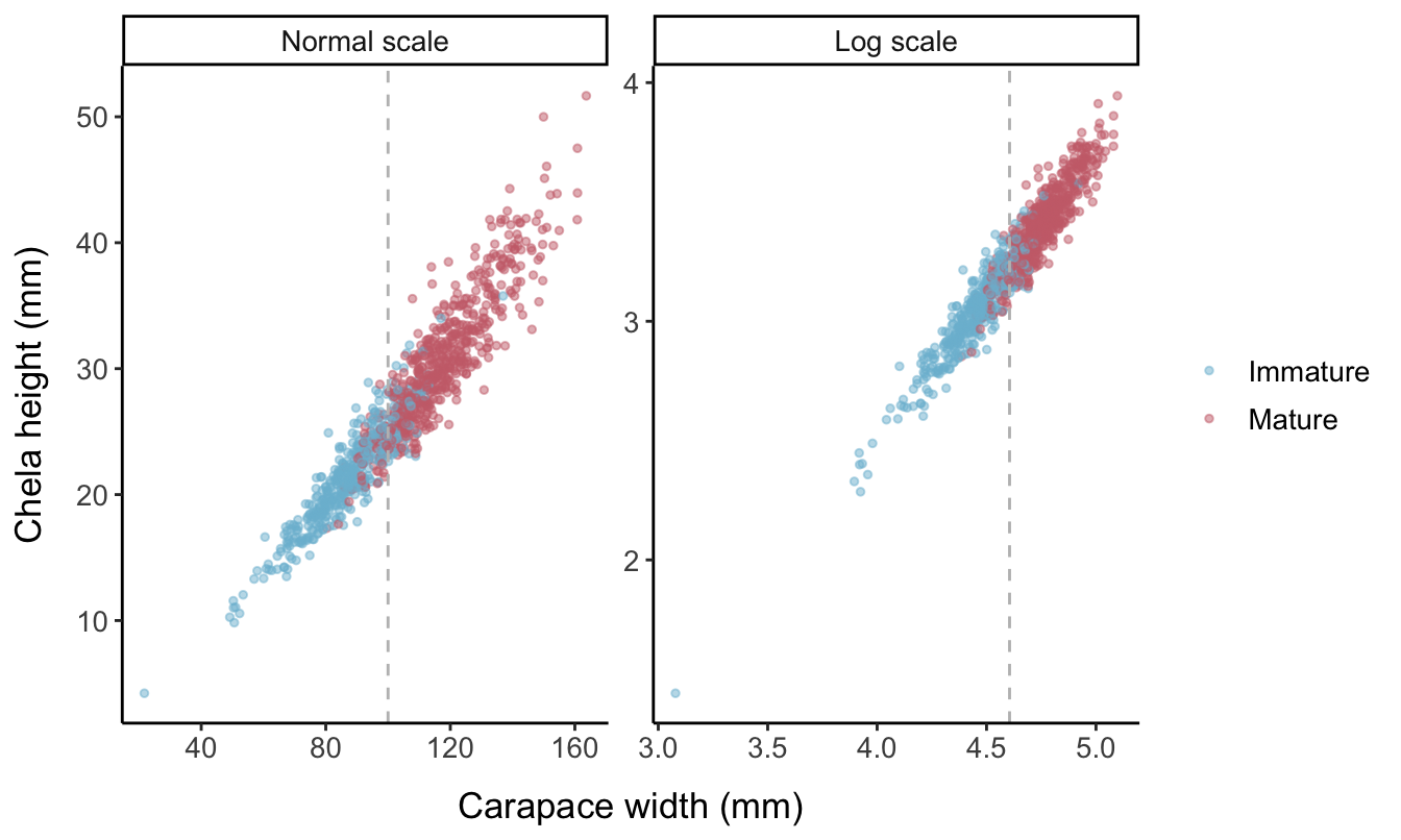
- Using given parameters for the slope and intercept of the allometric equation, find the predicted chela height for each individual based on their carapace width.
The allometric growth equation is \begin{equation}Y=\beta X^{\alpha},\end{equation}
which results in a linear plot when log-transformed: \(\log{(Y)}= \tilde\beta+\alpha \log{(X)}\). Here, \(\alpha\) is the slope of the allometric line and \(\beta\) is the intercept, with \(\tilde{\beta}=\log{(\beta)}\). Differences in the intercept of the allometry indicate differences in the proportionate size of the chela, irrespective of carapace width. In contrast, differences in the slope parameter represent differences in how the relative size of the chela changes with body size.
The fake_crustaceans default is no change in the allometric slope or intercept parameters \((\alpha=1.2, \beta=0.1)\) upon reaching maturity, so if this was real data, we would not actually be able to estimate size at maturity based on a change in morphometric ratios. The SD of the error distribution also remains constant upon reaching maturity.
- Add error representing individual variation in allometric growth. Errors added in Step 4 are assumed to be normally distributed around the regression lines obtained by log-transforming the raw CW and CH values. In other words, the data are assumed to have multiplicative log-normally distributed error:
\[Y=\beta X^{\alpha}e^{\varepsilon}, \quad \varepsilon \sim N(0,\sigma^2)\] \[\log{(Y)}=\log{(\beta)}+ \alpha\log{(X)}+\varepsilon, \quad \varepsilon \sim N(0,\sigma^2)\]
The question of whether error structures should be assumed to be multiplicative or additive when fitting allometric models is non-trivial and often controversial (Packard 2009; Ballantyne 2013; Xiao et al. 2011). However, the assumption of multiplicative error is often appropriate for biological contexts and in this case, simulating error based on a multiplicative structure generates artificial data sets that adequately resemble the empirical morphometric data sets we are interested in (Xiao et al. 2011; Kerkhoff and Enquist 2009). Variance in empirical size-at-maturity data often appears higher for mature individuals, so by assuming a multiplicative error structure, these errors will be proportional to the x-axis variable. For example, a measurement error of 4 mm would be less likely to occur when measuring a crab with a carapace that is 30 mm in length (a 13% error) than for a crab with a 100-mm carapace (a 4% error). Alternative error distributions for allometric models continue to be developed, and future extensions of our research could consider the performance of various size-at-maturity models when applied to simulated data with different forms of error (Echavarría-Heras et al. 2024).
References
Austin, M. P., L. Belbin, J. A. Meyers, M. D. Doherty, and M. Luoto. 2006. “Evaluation of Statistical Models Used for Predicting Plant Species Distributions: Role of Artificial Data and Theory.” Ecological Modelling, Predicting species distributions, 199 (2): 197–216. https://doi.org/10.1016/j.ecolmodel.2006.05.023.
Ballantyne, Ford. 2013. “Evaluating Model Fit to Determine If Logarithmic Transformations Are Necessary in Allometry: A Comment on the Exchange Between Packard (2009) and Kerkhoff and Enquist (2009).” Journal of Theoretical Biology 317 (January): 418–21. https://doi.org/10.1016/j.jtbi.2012.09.035.
Deroba, Jonathan J., D. S. Butterworth, R.D., Jr Methot, J. A. A. De Oliveira, C. Fernandez, A. Nielsen, S. X. Cadrin, et al. 2015. “Simulation Testing the Robustness of Stock Assessment Models to Error: Some Results from the ICES Strategic Initiative on Stock Assessment Methods.” ICES Journal of Marine Science 72 (1): 19–30. https://doi.org/10.1093/icesjms/fst237.
Echavarría-Heras, Héctor, Enrique Villa-Diharce, Abelardo Montesinos-López, and Cecilia Leal-Ramírez. 2024. “An Extended Multiplicative Error Model of Allometry: Incorporating Systematic Components, Non-Normal Distributions, and Piecewise Heteroscedasticity.” Biology Methods and Protocols 9 (1): bpae024. https://doi.org/10.1093/biomethods/bpae024.
Kerkhoff, Andrew J., and Brian J. Enquist. 2009. “Multiplicative by Nature: Why Logarithmic Transformation Is Necessary in Allometry.” Journal of Theoretical Biology 257 (3): 519–21. https://doi.org/10.1016/j.jtbi.2008.12.026.
Lotterhos, Katie E., Matthew C. Fitzpatrick, and Heath Blackmon. 2022. “Simulation Tests of Methods in Evolution, Ecology, and Systematics: Pitfalls, Progress, and Principles.” Annual Review of Ecology, Evolution, and Systematics 53 (1): 113–36. https://doi.org/10.1146/annurev-ecolsys-102320-093722.
Packard, Gary C. 2009. “On the Use of Logarithmic Transformations in Allometric Analyses.” Journal of Theoretical Biology 257 (3): 515–18. https://doi.org/10.1016/j.jtbi.2008.10.016.
Piner, Kevin R., Hui-Hua Lee, Mark N. Maunder, and Richard D. Methot. 2011. “A Simulation-Based Method to Determine Model Misspecification: Examples Using Natural Mortality and Population Dynamics Models.” Marine and Coastal Fisheries 3 (1): 336343. https://doi.org/10.1080/19425120.2011.611005.
Weber, Lukas M., Wouter Saelens, Robrecht Cannoodt, Charlotte Soneson, Alexander Hapfelmeier, Paul P. Gardner, Anne-Laure Boulesteix, Yvan Saeys, and Mark D. Robinson. 2019. “Essential Guidelines for Computational Method Benchmarking.” Genome Biology 20 (1): 125. https://doi.org/10.1186/s13059-019-1738-8.
Xiao, Xiao, Ethan P. White, Mevin B. Hooten, and Susan L. Durham. 2011. “On the Use of Log-Transformation Vs. Nonlinear Regression for Analyzing Biological Power Laws.” Ecology 92 (10): 1887–94. https://doi.org/10.1890/11-0538.1.